
NannyML has released DLE, an algorithm able to predict the MAE and the MSE of your regression model, in the absence of the ground truth
In a previous article, we have seen how to predict the performance of your classification model, before the ground truth is available. This is super useful in a real-world setting because it gives you early feedback about how your model is performing in production.
This was made possible by an algorithm conceived by NannyML, called “Confidence-Based Performance Estimation” (CBPE), which uses the probabilities predicted by the model to obtain a reliable estimate of any classification metric. A natural question is:
Can we do it also for regression models?
According to NannyML, yes, we can. They have developed a method called “Direct Loss Estimation” (DLE) that allows estimating the performance (specifically Mean Absolute Error and Mean Square Error) of any regression model, when the ground truth is not available.
They claim here that — as a one-stop solution to estimate performance — DLE outperforms other approaches, such as Bayesian method or Conformalized Quantile Regression. But until we don’t see we don’t believe, right? So, in this article, we will explore DLE, try it on a real dataset, and see if it actually performs well as NannyML promises.
The main idea
The intuition behind DLE is very simple. So simple that it seems too good to be true. Basically, the idea is to directly predict the errors made by the model.
I know what you are thinking. You are probably skeptical because you’ve heard that:
“You cannot make a model predict the errors of another model.”
But is it true? To answer this question, we need to start from the posterior distribution.
Introducing the posterior distribution
We are used to models that return a single value for each observation, also called “point prediction”. However, we must keep in mind that, behind that point prediction, there is always a full distribution. If you like fancy statistical terms, you can call this the “posterior distribution”.
What’s the meaning of the posterior distribution?
The posterior distribution gives you a full account of the uncertainty of the prediction.
Let’s try to understand it with the aid of an example.
Suppose that we trained a model to predict the income of a person based on her country, gender, age, marital status, and job. Now, imagine that we have 10,000 people, all with the following characteristics:
- Country: USA.
- Gender: Female.
- Age: 27.
- Marital status: Married.
- Job: Salesperson.
Of course, even though they carry the same features, they will not have the same income. We can imagine the distribution of their incomes as the posterior distribution for this particular combination of features.
Let’s generate a posterior distribution in Python:
# generate posterior distribution

import numpy as np

posterior_distribution = np.random.lognormal(0, .25, 10000) * 50000
This is the histogram of the distribution:
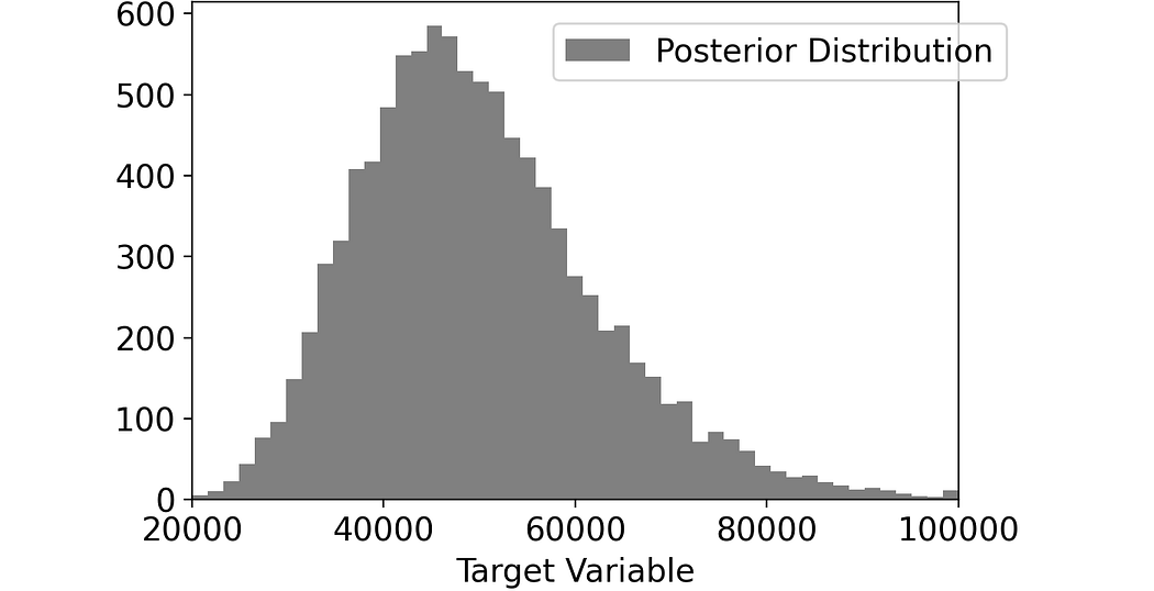
The cool thing about knowing the posterior distribution is that we can calculate anything we want: percentiles, mean, median… Anything.
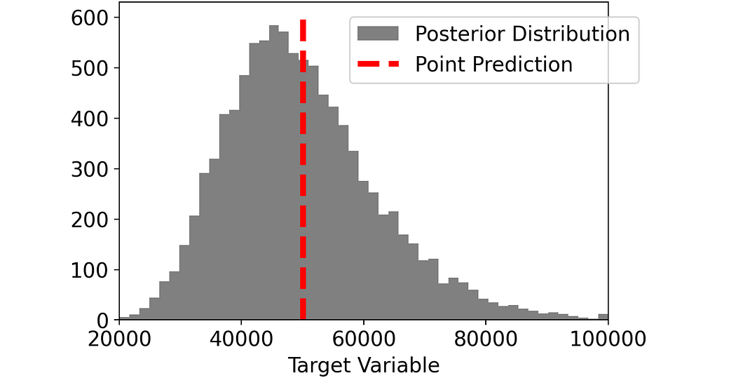
However, most predictive models are designed to get a point prediction. Indeed, when given the 10,000 individuals above, your model will predict the same income for each of them. As you can guess, the models are usually designed to predict the mean of the posterior distribution.
np.mean(posterior_distribution)In our case, this is 50,000 $. So, this is the model’s prediction.
Why it doesn’t make sense to predict the error…
For each one of our individuals, the error is given by the difference between the point prediction and the true value. For example, if the income of a person is 65,000 $, the error made by the model is -15,000 $.
error_distribution = point_prediction - posterior_distributionAnd if you take the mean error:
mean_error = np.mean(error_distribution)This is of course zero by definition.
The fact that the mean error is zero makes a lot of sense. It means that, on average, our model makes the right predictions, because positive errors balance out negative errors.
At this point, it’s easy to see why it doesn’t make sense to predict the error. Because it would mean trying to predict something that is null by definition. ***
But didn’t we say that DLE is based exactly on predicting the error? So, what’s the catch?
*** We are assuming that the model predicts the mean of the posterior distribution. This is not always the case. For example, if you use a loss function different from MSE, your errors may not be 0-centered. However, in that case, predicting the signed error would still be pointless: it would be like “correcting” the loss function that you chose in the first place.
… But it makes a lot of sense to predict the absolute error
The point is that DLE does not predict the signed error, but the absolute error!
It may seem like a small difference, but actually, it’s a whole different story. In fact, contrary to the signed error:
The absolute error is a measure of how uncertain our point prediction is.
Having the posterior distribution, we can compute the absolute errors:
absolute_error_distribution = np.abs(point_prediction - posterior_distribution)And if we take the mean, we get the mean absolute error:
mean_absolute_error = np.mean(absolute_error_distribution)
With the distribution we have simulated, the mean absolute error is around 10,000 $. It means that, on average, the actual income is 10,000 $ away from the point prediction given by our model.

To sum up:
- Trying to predict the signed error makes no sense, because we are trying to correct a model that we believe to be the best one.
- Trying to predict the absolute (squared) error makes a lot of sense, because we are trying to quantify the uncertainty associated with the prediction.
Note that the final performance of our model is directly linked to the uncertainty associated with it. It’s intuitive. The more uncertainty, the worse performance. The less uncertainty, the better performance.
Describing DLE algorithm
In practice, DLE trains a new model that learns the uncertainty associated with the predictions of the original model. In fact:
- The original model makes the point predictions (as always).
- The model introduced by DLE predicts the absolute (or squared) errors made by the main model. NannyML calls this one “nanny model” (for obvious reasons).
We can summarize the whole process in 4 steps.
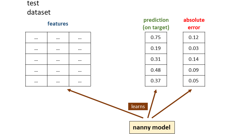
As usual, everything starts with training the model on the training dataset.
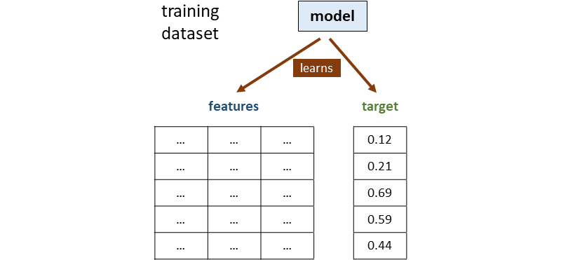
Then, the model is used to make predictions on the test dataset. Once we have the predictions, we can also calculate the absolute errors as the absolute difference between target and prediction:
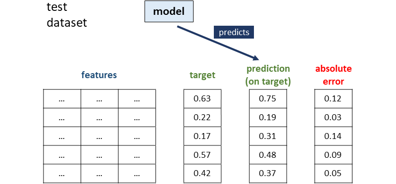
At this point, a second model — called the nanny model — uses the original features and the predictions made by the first model to learn patterns about absolute errors.
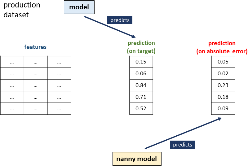
Finally, when the model is used in production to make predictions, we can use the first model to predict the target variable and the nanny model to predict absolute errors.
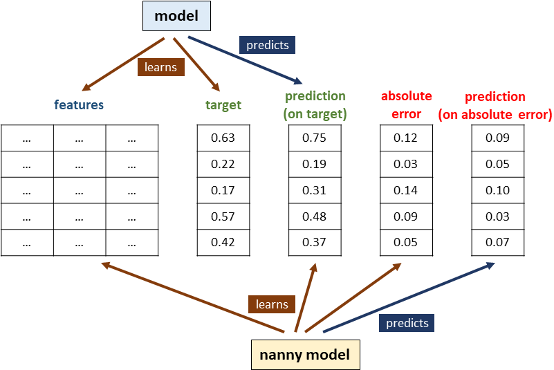
To summarize, this is a view of the entire process (with no distinction between training, test and production datasets for clarity):
Predicting performance on a real dataset
Let’s see if DLE works on a real dataset.
We will use the Superconductor dataset, an open-source dataset from UCI. This dataset consists of 21,263 materials, with 81 features recorded regarding atomic mass, atomic radius, density, and others. The goal is to predict the critical temperature.
We will split the dataset into a training, a test, and a production dataset.
# load data and split into train, test, prod

import pandas as pd

df = pd.read_csv("/kaggle/input/superconductor-dataset/train.csv").sample(frac=1, random_state=123)

df_train = df.iloc[:int(len(df)/5)]
df_test = df.iloc[int(len(df)/5):int(len(df)/5*2)]
df_prod = df.iloc[int(len(df)/5*2):]

X_train = df_train.drop("critical_temp", axis=1)
X_test = df_test.drop("critical_temp", axis=1)
X_prod = df_prod.drop("critical_temp", axis=1)

y_train = df_train["critical_temp"]
y_test = df_test["critical_temp"]
y_prod = df_prod["critical_temp"]
At this point, we are ready to train our model:
# train model

from lightgbm import LGBMRegressor

model = LGBMRegressor().fit(X=X_train,y=y_train)
Then, we use the test dataset to compute the errors made by the model.
# compute observed errors made by the model on test data

pred_test = pd.Series(model.predict(X_test),  index=X_test.index).clip(0)

error_test = pred_test — y_test
Once we have the errors, we can train the nanny model. Note that the nanny model uses as features all the original features plus the predictions made by the first model.
# train model to predict the absolute error

model_abs_error = LGBMRegressor().fit(
  X=pd.concat([X_test, pred_test], axis=1),
  y=error_test.abs()
)
On the production dataset, we first use the main model to obtain the predictions. Then, we use the nanny model to get the predicted absolute errors.
# predict the absolute errors on production data

pred_prod = pd.Series(model.predict(X_prod), index=X_prod.index).clip(0)

pred_abs_error_prod = pd.Series(model_abs_error.predict(pd.concat([X_prod, pred_prod], axis=1)), index=X_prod.index)
At this point, we have the prediction of the absolute error for every single observation. Thus, we can finally predict the Mean Absolute Error (MAE) on the production dataset, which was our initial goal.
# predict MAE on production set

pred_mae_prod = np.mean(pred_abs_error_prod)
Testing DLE against data drift
The whole purpose of DLE is to predict the MAE (or MSE) of our model when we don’t have the ground truth. This is extremely useful in a real-world scenario when we want to know in advance if there is a deterioration in the performance of our model.
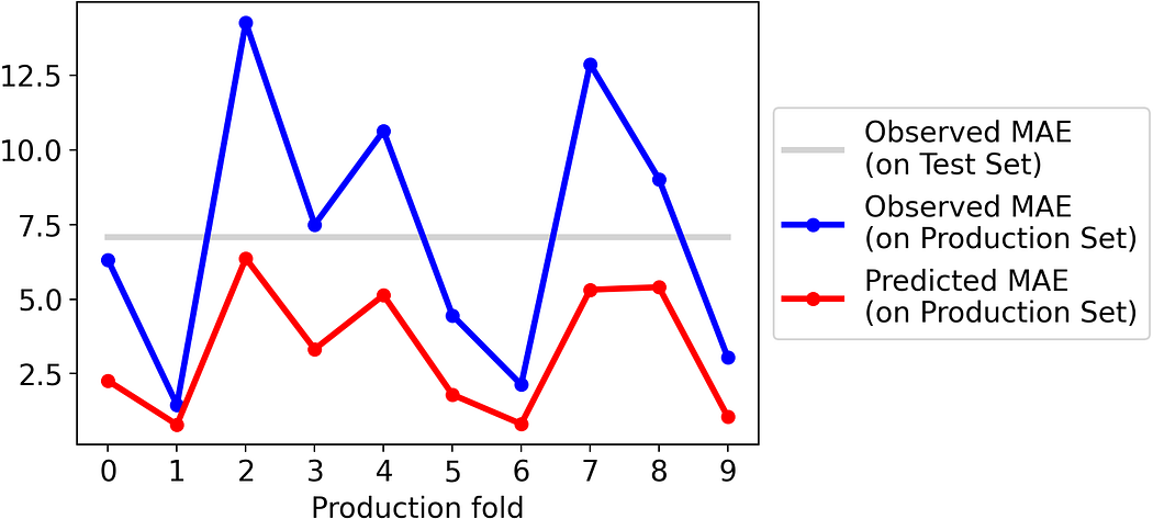
In order to simulate this scenario, we will split the production set into ten folds. To reproduce data drift, we will not split the folds randomly, but we will divide them based on the predictions made by the model. In this way, we make sure that the folds are sufficiently different from each other, and that the performances are reasonably different across the folders.
So, let’s compare the actual MAE on each folder with the MAE obtained as the mean of the absolute errors predicted by the nanny model.
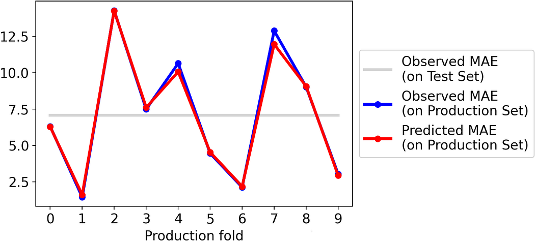
The results are impressive. The MAE predicted through the nanny model is practically the same as the actual MAE.
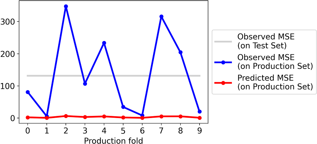
Let’s try with the MSE:

Also in this case, the results are amazingly good.
What happens if we try to estimate the error (rather than the absolute error)?
We have already seen above that trying to estimate the signed error makes no sense, from a theoretical point of view. But since data scientists prefer the practice over the theory, let’s try to do it anyway.
In other words, this means repeating the procedure above but, rather than training the nanny model on test absolute errors, training it on test signed errors.
Translated in Python, this means the following:
# train model to predict the error (which makes no sense)

model_error = LGBMRegressor().fit(
  X=pd.concat([X_test, pred_test], axis=1),
  y=error_test
)
Now, we are able to get a prediction of the signed error for each observation in the test set. If we take these predictions, take their absolute value, and then average them, this is a new estimate of the MAE.
Let’s see how it would perform on the same test folds as above:
It’s evident how, using this new strategy, the predicted MAE systematically underestimates the actual MAE.
This is even worse if we try to do it for MSE:
This is just further proof that predicting the absolute error is completely different from predicting the signed error and then taking the absolute error.
And if you don’t want to reinvent the wheel…
In this article, we have implemented DLE from scratch to show how it works under the hood. However, in real life, it’s often preferable to use libraries that are well maintained.
So, you may want to directly use NannyML, which has several native functionalities, such as fitting hyperparameters for you.
# use DLE directly with NannyML

import nannyml as nml

estimator = nml.DLE(
  feature_column_names=features,
  y_pred='y_pred',
  y_true='critical_temp',
  metrics=['mae', 'mse'],
  chunk_number=10,
  tune_hyperparameters=False
)

estimator.fit(df_test)

results = estimator.estimate(df_prod_drifted)
Moreover, you can easily obtain fancy plots about your model performance with one line of code:
results.plot(metric=’mae’)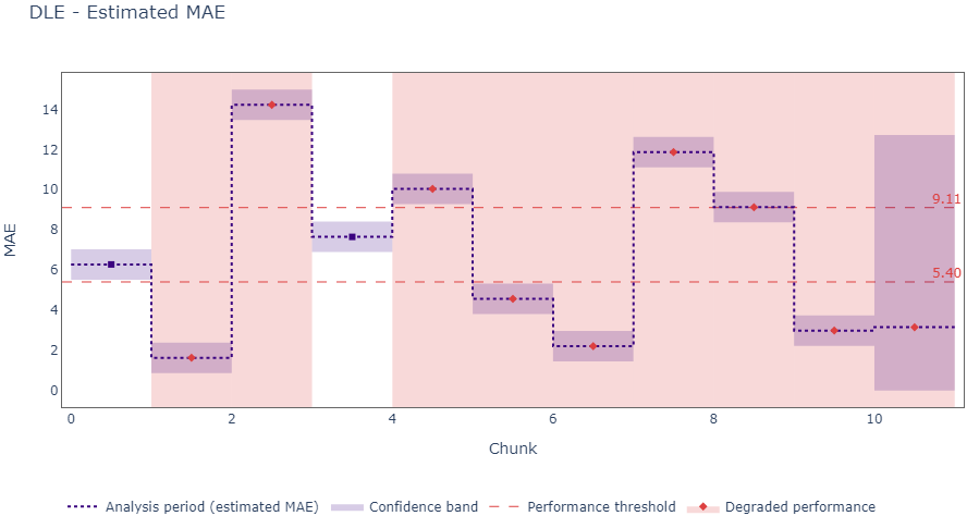
When it won’t work
When using DLE to estimate performance, there are some assumptions that you should pay attention to. Indeed, if some of these assumptions are violated, the performance estimated by DLE may not be reliable anymore. These are the assumptions:
- There is no concept drift. If the relation between the features and the target variable changes in unforeseen ways, the error that you are trying to predict changes as well, and so the nanny model may fail.
- There is no covariate shift to previously unseen regions in the input space. Both the main model and the nanny model learn on the original features. If the features drift to values not seen during the training/validation phases, the models may make an uncorrect guess.
- The sample of data is large enough. Of course, both the training and the validation dataset need to be large enough for both the models to be robust.
Summing up
In this article, we have seen how to reliably predict the expected performance (specifically, MAE and MSE) of a regression model, when the ground truth is not available.
This algorithm — called “Direct Loss Estimation” (DLE) — has been proposed in this article by NannyML (an open-source library focused on post-deployment data science).
DLE is based on the intuition of directly predicting the absolute (or the squared) error of each single observation. We have tested it on the Superconductor dataset and obtained outstanding results.
You can find all the code used for this article in this Github repository.
Thank you for reading! I hope you enjoyed this article. If you’d like, add me on Linkedin!
This article was originally published in Towards Data Science.


Comments